Richard Gage Blueprint for Truth Rebuttals on YouTube by Chris Mohr

[Christopher7]

Nope, I am not a metallurgist. But, you do make the claim, so you back it up. Show me that A-Thermite or nano thermite produces oxygen rich spheres, (No, the John Cole video is not proof of that. ) and B-That is unique to a thermite reaction.

Page 17 of the thermite paper.

 

[femr2]

It would take an external force pushing down to achieve greater than g for over a second.

A force pulling is rather more practical, such as the building core. Remember that the trace is for the NW corner of the building. Remember that during the period of over-g, the NW corner only descends about 50ft. Remember that the data is not exact, with magnitude being one potential error source. ie the vertical scale "may" be slightly out. It's at the mercy of scant building metrics from NIST, and physical measurement of building features taken from video after all. All done with the greatest of care, but certainly a potential source of error. There's no reason for me to doubt my data, and numerous reasons why a period of over-g could be expected.

Remember that the NIST acceleration profile also contains a period of over-g.

The interior columns falling at FFA cannot make the exterior columns fall at greater than FFA for more than an instant.

Of course they can. Simplest way of looking at it could be the core giving the NW corner a sharp tug. It wouldn't then instantly revert to ~ffa, but would take a short time, which is what is seen in the graphs.

NIST and a physics teacher with two masters degrees agree that WTC 7 fell at FFA for 2.25 seconds.

lol. NISTs own data doesn't agree with that statement. Only NIST wrote the 2.25s summary. Chandler came up with a different value. In other words, they don't agree. Both are averages, not AT. Both are inaccurate and based on crap data which was extracted with little care and poor understanding of of the "field". If you wish, I'll point you to the extensive lists of reasons here which explain WHY their datasets are severely flawed if you like. That may reduce the impotent hand-waving you seem to be engaging in.

FEMR's graphs are junk science.

They're the best you're going to get, and are far superior to and more accurate than those others you keep mentioning.

Btw, who do you think had the correct data ? NIST or Chandler ? Their datasets are quite different you know

 

[Oystein]

My bad, that's what I meant. I reposted it in a hurry after my browser crashed when I had it written properly and got the term reversed the second time around. Sorry.

So, I've been wondering if the endothermic peak might be the result of the melting of the steel layer. Is that possible?

More exactly, the endothermic peak seen in some of the samples.

Which ones?? In these graphs, endothermic "peaks" would actually be troughs:

Are you thinking of the troughs near 410°C of the two MacKinlay samples (red and blue)?

Quite likely these represent some phase change - but I don't think that the iron oxide is involved here; much more likely it's some transition within the organic matrix, perhaps some evaporates, or a glass transition. An endotherm chemical reaction has also a non-zero possibility, but without even knowing what materials went into that reaction, it is impossible to speculate with any degree of confidence at all what it might have been.

ETA: Urrr I just looked at the graphs after I posted, and it struck me immediately that even these "troughs" have positive values for heat release, so they are exotherm, not endotherm. They could be some endotherm process superimposed on the larger exotherm reaction, or a separation between two distinct exotherm peaks. Difficult to tell, due to the incompetent description of the test procedure and input materials.

However, the Intermont and White samples (green and black) dip into enotherm territory beyond 570°-620°C and stay there till 670-680°C, roughly. That could easily be melting or evaporation of something. (The melting point of aluminium, 660°C, happens to be smack dabble in that range - so is this possible proof of elemental aluminium? Well, for starters, no, it really could be a thousand things. But if there was so much Al as to significantly imprint its melting on a DSC curve, then where is it after the reaction, where was it before, and why wasn't it consumed in the thermite reaction if that is such high-grad nano-tech superduper stuff?? )

 

[Oystein]

They don't discuss the aluminum oxide as far as I can see. So what? That does not mean there wasn't any.

Uhm Tillotson and Gash explained in their paper that they took pains to actually analyse the residue to ascertain that a thermite reaction had in fact taken place by using PXRD to demonstrate the presence of Al2O3. They did NOT do the DSC test to proof it was a thermite reaction - they did the PXRD proof for alumina.
That's precisely what Jones e.al. did NOT.

YOU claimed that white alumina smoke was ejected from the reaction, yet you are not worried that there is no mention of it. I find that interesting and telling.

They did say this: "Other iron-rich spheres were found in the post-DSC residue which contained iron along with aluminum and oxygen (see Discussion section)".

Exactly. They do NOT say that they found any appreciable amount of iron oxide. Strange, eh?

The white smoke comment was made elsewhere.

Oh yes? Link please!

Smoke can be particulate matter as well as gases so the aluminum did not have to evaporate as pgimeno was suggesting. Example of white smoke @ 0:04
http://www.youtube.com/watch?feature=player_embedded&v=S1TwVACENAo

White smoke? I say grey smoke, or perhaps condensed steam. Not white smoke. How can you say what material is ejected there without an analysis? I plan on cooking something later. If my food ejects stuff that looks similar to this, will you agree I'll have thermite residue for dinner?

Chris7, this is Mark Basile's "lucky" chip 13. Here is his quantitative analysis of the elemental composition before burning:

Do you see how he only has less than 1.7% Al in the red layer of that chip to start with, but around 3% other metals? And how he has >70 carbon, which translates to something like 88% organic matrix (hydrocarbon), which is almost certainly combustible and almost certainly burns before any thermite would? So how can you rule out that the smoke (or condensed vapor) you see in that video is not any other mineral dust, or the products of some organic reaction like - H2O or soot? Did Basile do ANYTHING to ACTUALLY prove alumina?

It's the average. My use of the word "suddenly" was incorrect.

Nice try. Too bad you were caught

The reaction took place between 370^oC and 470^oC

Yes. At a heating rate of 10°C/minute, that reaction took place over the course of how many minutes? (Hint: 370-470°C is a span of 100°C. Divide that by the heating rate: 100/10. Use a pocket calculator, if you can't do it in your head. Please provide the result in a full sentence: "The exotherm reaction observed when Farrer burned several micrograms of tests of red-gray chip samples DSC lasted approximately ____ minutes. This is a very sudden/fast/intermediate/slow reaction speed").

Please, we are talking about the red/gray chips, not building materials.

Incorrect. We are talking about steel primer, which is a building material.

 

[MarkLindeman]

Aiii. I hope I've shown that even the poly(10) end result exhibits the same general profile as the far superior S-G acceleration derivation.

Sure. But, I missed the Great femr2 Wars. I'm just looking at poly(10) and thinking, "Gee, why use poly(10)?" I don't want to get hung up on that one way or another; it's like debating whether Bazant and Zhou has been ``refuted.''

I've performed numerous tests, one of which may be of interest...
http://www.internationalskeptics.com/forums/showpost.php?p=6114713&postcount=232

That's really very cool. It's not, however, what I had in mind by sensitivity analysis. If, for instance, you think that all things considered, your measurements are subject to +/- 0.2 pixel errors -- I'm not sure what your basis for that was, but I'll stipulate it -- then one approach to sensitivity analysis (which you may already have done) is to model some simulated data that model that error, add it to your observations, and fit the acceleration curves accordingly. For instance, you might generate 1000 data sets where you add an error term that is N(0, 0.1px) (ETA: or whatever seems reasonable in that regard) -- or maybe it makes more sense for the error terms to be autocorrelated. Then the ``envelope'' of the resulting acceleration curves would give some additional insight into the robustness of your qualitative findings (cf. below). Of course it's possible that the error is greater during the collapse, but if someone wants to argue that, s/he should actually have an argument.

I realize that some people here are eager to find an excuse for your qualitative findings to go away. I'm not. I'm not heavily invested in your findings one way or another, but they seem pretty solid to me: intuitively, the ``jitter'' already gives considerable insight into the effect of measurement error. I do prefer to have some explicit estimate* of error, rather than my own eyeballed guesstimates alone. In this case, it might give some insight into whether some parts of the acceleration curve are estimated with more error than other parts. I wouldn't expect that to influence the qualitative conclusions, but it might nonetheless be informative.

*(ETA) Of course the estimate is subject to debate, and that is one element of sensitivity analysis: Just how sensitive are the results to assumptions about measurement accuracy? That's an empirical question.

 

[triforcharity]

Page 17 of the thermite paper.

Which doesn't address my two questions at all.

Please feel free to try again.

 

[carlitos]

Pity their trace data results were so shoddy really. The havok caused by their published words was really unneccesary, and could have been avoided if they had applied a little more time/effort/focus. Poor. It's not rocket science.

The havoc caused was entirely in the imagination of the "truth" movement.

I have to agree on the highlighted bit, but not on the corrective action. It was a really unnecessary study, with some hallmarks of being made in a hurry (as in, "let's put something together quickly to address this" without really caring about the quality of the final result), and what for? Just as a reply to purely accessory criticism. The influence on their conclusions? Zero. The focus of the report is, as it should be, on the initiation mechanism.

I'd disagree with your highlighted bit, but agree with your overal conclusion.

 

[NoahFence]

Aren't the red and grey chips part of the building materials?

 

[MarkLindeman]

Not to sound arrogant or anything, but those of us who are "truthers" (or those who, at the very least, question the official story ) should try to avoid this type of thing.... I mean the reality is there really is no need to do measurements at all. All one had to do is watch the video a WTC7 to know it was a CD. If WTC7 was rigged, there is no doubt the towers were as well.

Actually, those of you who are "truthers" should try to avoid this type of thing. Right here. This.

 

[beachnut]

Sure. But, I missed the Great femr2 Wars. I'm just looking at poly(10) and thinking, "Gee, why use poly(10)?" I don't want to get hung up on that one way or another; it's like debating whether Bazant and Zhou has been ``refuted.''
...

There are is no value in study of the collapse past what NIST gathered. The study of the collapse of a single point is good for what? Exactly, there is not thesis, no goal, and no ability to state what the same looking curve shape has to do with anything. The same basic shape is found for NIST and femr2 "best" work. What is the purpose of the data?
This is typical of femr2, where he learns as he goes. He does not like NIST. Where does this bashing NIST come from? Who cares about NIST?

femr2 on NIST - We are asked to believe that 2,966 gallons of jet fuel, essentially kerosene, caused the collapse of the South Tower.

NIST never said that, and in this case of the "best" data for collapse time/speed/acceleration what is the purpose, and what is the conclusion. How does this change NIST's conclusion on the probable collapse, as in probable?

Why goals? Before I go off with Don Quixote, I would like to know the big picture; not that I don't like going along, but some days I enjoy purpose driven quests.

What is the reason you seek the cup of Christ? In this case study of time/speed/acceleration is a waste of time since a rough estimate is all that is needed. The cool part, NIST was not looking to back in CD like the failed 911 truth movement.

Someone, please explain why the rough estimate NIST has is not adequate for the task? Goals for femr2's work? How his work changes anything?

I don't need NIST; most engineers would do their work and ignore NIST, make conclusions.

 

[femr2]

I'm just looking at poly(10) and thinking, "Gee, why use poly(10)?"

Simply tools I had to hand at the time. Previously I'd used all manner of running-average-like methods, so the general profile was "known", and the poly(x) results were simpler to look at, but well fitting. Savitzky-Golay has definitely supersceded all prior smoothing methods (though I do/did employ 2-sample running average when recombining per-field traces back together.

That's really very cool. It's not, however, what I had in mind by sensitivity analysis.

Of course.

A more "real world" example...

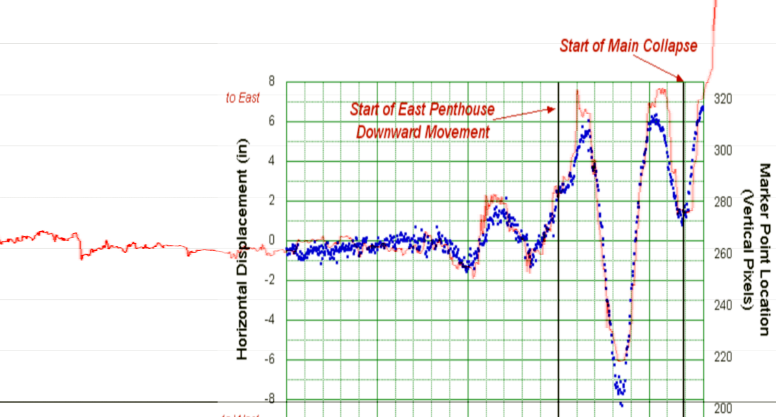
My data (red). NIST data (blue). Note the displacement scale...inches.

Worth noting that NIST used a different (and much less accurate) method for their descent trace. I used the same trace method for all trace points (SynthEyes - x8 upscale with LancZos3 filtering on separated fields).

As an aside, WTC7 images are here.

If, for instance, you think that all things considered, your measurements are subject to +/- 0.2 pixel errors -- I'm not sure what your basis for that was, but I'll stipulate it

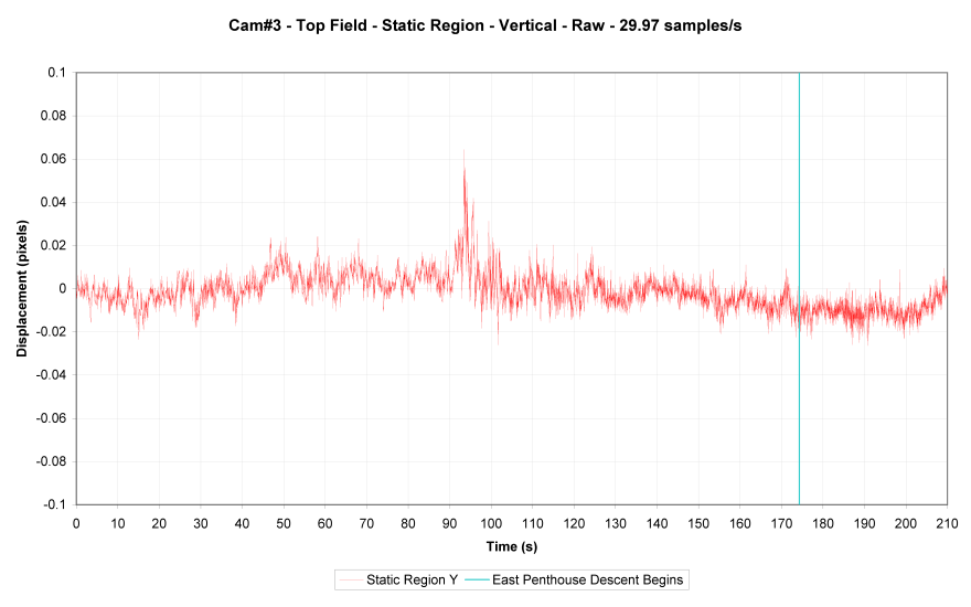
It was based upon the variance of static point positional data, and trace point variance during static periods...and was a very early value. Latter more refined traces contained lower static point positional variance...

...nearly an order of magnitude improvement.

Additional noise sources are present of course. I'd have to wade through old posts to find the specific dataset from which the +/-0.2pixel variance was determined, but I'm happy for it to stand.

one approach to sensitivity analysis (which you may already have done) is to model some simulated data that model that error, add it to your observations, and fit the acceleration curves accordingly. For instance, you might generate 1000 data sets where you add an error term that is N(0, 0.1px) (ETA: or whatever seems reasonable in that regard) -- or maybe it makes more sense for the error terms to be autocorrelated. Then the ``envelope'' of the resulting acceleration curves would give some additional insight into the robustness of your qualitative findings (cf. below). Of course it's possible that the error is greater during the collapse, but if someone wants to argue that, s/he should actually have an argument.

Sure. It's useful to know that measurement error is relative to an absolute position. Smoothing was applied to the raw displacement/time data before derivation of velocity and acceleration. A full error analysis has not been performed. I'll dig out what was done when I find it.

the ``jitter'' already gives considerable insight into the effect of measurement error.

Jitter you mention may be that caused by recombining upper and lower field traces. Such jitter is effectively removed by a simple 2-point rolling average (or similar). Static point trace above should give you an idea of what became possible.

it might give some insight into whether some parts of the acceleration curve are estimated with more error than other parts. I wouldn't expect that to influence the qualitative conclusions, but it might nonetheless be informative.

Sure. My personal focus is the trend/shape, rather than absolute magnitude, but many traces, many viewpoints, many smoothing methods all end up with similar results. Without significant reason I'm probably unlikely to invest the time.

 

[LSSBB]

You are the one making that claim, you prove that it can happen. Don't ask me to prove a negative.

You are the one that said it is impossible. Back up what you say.

 

[LSSBB]

Chris, this should help put things into perspective. Think about the force the interior collapse is putting on the perimeter, and then what happens when the perimeter columns fail near the base (probably assisted by interior debris spreading) and the resistance drops down to much less than g force.

 

[MarkLindeman]

There are is no value in study of the collapse past what NIST gathered.

What is wrong with good old-fashioned curiosity? We don't have to reduce every single thing to a salvo in Truthers v. Debunkers.

That said....

The same basic shape is found for NIST and femr2 "best" work. What is the purpose of the data?

Since when is independent replication a bad thing?

This is typical of femr2, where he learns as he goes.

Yes. Ain't it grand? Whatever disagreements I may have with femr2 -- and I imagine there are many -- I certainly won't criticize anyone for learning as s/he goes. If everyone did that, maybe this forum wouldn't feel so much like Groundhog Day.

Someone, please explain why the rough estimate NIST has is not adequate for the task? Goals for femr2's work? How his work changes anything?

Hey, watching one of the other forum members squirm is rationale enough for me. I think it's hilarious.

Beyond that, I don't think the analysis is likely to be very consequential, but that's OK. The tools may be useful for some other problem.

My personal focus is the trend/shape, rather than absolute magnitude, but many traces, many viewpoints, many smoothing methods all end up with similar results. Without significant reason I'm probably unlikely to invest the time.

That's fair. This may not be the best test case for error analysis anyway, especially because the discussion is so weirdly polarized.

 

[beachnut]

What is wrong with good old-fashioned curiosity? We don't have to reduce every single thing to a salvo in Truthers v. Debunkers. ...

Nothing is wrong with curiosity driven by knowing 911 was an inside job and CD. I love faith based goal-free attacks on NIST.
Classifying attacks on NIST as curiosity does make it seem more, something. And of course there is the curiosity of labeling your videos "WTC Demolition", very curious.
I don't know how to appease ignorance and false claims based on the curiosity approach.

Since when is independent replication a bad thing? ...

The goal was not to verify, it was to find a way to back in the Demolition nonsense. Bad thing?

I don't know - what is this nonsense of attacking NIST? I would publish my findings. What was the purpose of doing the study, since a look at the video and the data NIST has is all that is needed; I have dividers, a ruler, a 110 inch screen, done in a few mintues.
Why the attacks on NIST? Curiosity?

Pity their trace data results were so shoddy really. The havoc caused by their published words was really unnecessary, and could have been avoided if they had applied a little more time/effort/focus. Poor. It's not rocket science.

Havoc? No one was killed in WTC 7. Fire safety, it worked, you leave building on fire; a lesson learned a long time ago.

Yes. Ain't it grand? Whatever disagreements I may have with femr2 -- and I imagine there are many -- I certainly won't criticize anyone for learning as s/he goes. If everyone did that, maybe this forum wouldn't feel so much like Groundhog Day. ...

I meant, learning late, spreading nonsense, then having to erase your words to cover-up jumping the gun. It is more like trying not to learn, being told the correct answer and ignoring it. No big deal, if he wants to call his youtube videos "WTC Demolitions", why worry about misleading the next Tim McVeigh; who cares? Drum up some more attacks on NIST.

Beyond that, I don't think the analysis is likely to be very consequential, but that's OK. The tools may be useful for some other problem. ...

 

[MarkLindeman]

Nothing is wrong with curiosity driven by knowing 911 was an inside job and CD. I love faith based goal-free attacks on NIST.

Look, bottom line: femr2 did a detailed analysis that dovetails with NIST's conclusions on important points, and you seem every bit as ticked as if he(?) had written a nonsensical defense of Chandler. I'm happy to disagree with femr2 about all the things that we actually disagree about, but I don't see a reason to haul them into this thread -- even if I kept a file, which I don't.

 

[pgimeno]

Remember that the NIST acceleration profile also contains a period of over-g.

That can't be stressed enough to C7, who is claiming all the time that the average ~g acceleration measured by NIST has to be regarded as instant acceleration sustained over time.

 

[pgimeno]

Which ones??

I was wondering about the ones at 640-660°C in Mackinlay2 and Intermont (black/green). The gray layer was not nano-sized, so I don't expect its melting temperature to be in the 400°C range.

The melting might well happen during the burning, I was just considering other possibilities.

Hmmm... wait. If some of the heat was absorbed in melting the iron, that means that the peaks would be even higher if the iron wasn't there. My, that's a lot of energy. Thermite isn't that energetic.

 

[pgimeno]

Yes. At a heating rate of 10°C/minute, that reaction took place over the course of how many minutes? (Hint: 370-470°C is a span of 100°C. Divide that by the heating rate: 100/10. Use a pocket calculator, if you can't do it in your head. Please provide the result in a full sentence: "The exotherm reaction observed when Farrer burned several micrograms of tests of red-gray chip samples DSC lasted approximately ____ minutes. This is a very sudden/fast/intermediate/slow reaction speed").

B...

(arcs a brow)

O...

(looks at wrist watch)

(taps fingers)

O...

(grows impatient)

(rests chin in hand)

O...

(goes for a coffee)

...

(returns with the coffee)

O...

(drinks coffee slowly)

O...

(looks at watch again... 9 minutes...)

...M!!!!!!!!!!!!!!


Just so C7 can be sure of the source:

The DSC tests were conducted with a linear heating rate of 10 °C per minute up to a temperature of 700 °C.
​

(from the Bentham paper, p.10)

 

[pgimeno]

The white smoke comment was made elsewhere. Smoke can be particulate matter as well as gases so the aluminum did not have to evaporate as pgimeno was suggesting.

Add "evaporate" (or "eject" if you prefer) "only the aluminium oxide", even if should be majority by volume, to the magic properties of that thermite. The list is long by now.