• Quick note - the problem with Youtube videos not embedding on the forum appears to have been fixed, thanks to ZiprHead. If you do still see problems let me know.

Merged Discussion of femr's video data analysis

WD Clinger, considering the obvious flexure in the perimeter that the NIST fails to account for and the obvious differences between the NIST and femr accelerations during the inital and "greater than g" movement, aren't you starting to figure something out yet?

The NIST spreads out their early acceleration by ignoring the horizontal motion in the perimeter. Why can't you see that?
 
Last edited:
The NIST spreads out their early acceleration by ignoring the horizontal motion in the perimeter.
I'd say rather that NIST included the early motion as vertical, though with the same end result.

Note that, logically, swapping dataset from NIST to mine doesn't significantly affect the output curve, as the same formula is applied...
danA.png


It's amazing what can be concluded when noise...
82136974.png

...isn't pummelled a little, though the trend is still visible.
(Running Average and Wide-Band Symmetric Differencing only)

Makes one wonder what the relevance of computing Residual sum of squares against utterly unsmoothed data actually is. Makes you wonder if that is where the fubar is arising.

Makes me wonder if W.D.Clinger is fully aware of that noisy little nugget.

Now I have an acceleration trend summary...
513801604.png

...I'll probably do the same for velocity. No rush though.
 
Last edited:
femr: "I'd say rather that NIST included the early motion as vertical, though with the same end result."

I didn't phrase it carefully. They detected the earliest motion, which was horizontal, and thought it was purely vertical.

This creates the "stretching" of acceleration in their graph relative to yours. You didn't make that mistake because you were aware of the two components of motion and chose the Dan Rather clip for that reason.


Here is a nice model that shows this type of spring motion:

c3view.gif


topview.gif


From the camera 3 angle, If you are not careful to note the horizontal flexing during the earliest motion there is no way you can properly determine early acceleration.


Femr nailed it. NIST failed it. That is the difference.
 
Last edited:
...Makes one wonder what the relevance of computing Residual sum of squares against utterly unsmoothed data actually is. Makes you wonder if that is where the fubar is arising...
I'm 'one of the ones' who is made to wonder. I still haven't got my head around that one. :confused: The rest of the discussion is pretty transparent. I must be gettin' old or summat. :o
 
I'm 'one of the ones' who is made to wonder. I still haven't got my head around that one. :confused:
Do you mean (as I do) that the residual sum of squares value would be pretty nonsensical without performing it upon data which has been through noise reduction processing ?

The rest of the discussion is pretty transparent.
Could you elaborate ?
 
Last edited:
That would do it -- if the lens were perspective-free (or at an infinite distance).

One could also choose a reference point that, being near the center of the "kink," shows little or no left-right movement from any viewpoint and therefore could not have moved a great deal north-south.

Sorry, details whose relevance has not been established are difficult to remember after months. I have read the thread but in the absence of a coherent thesis it's difficult (and entirely unnecessary) to keep it all straight.

Respectfully,
Myriad
Early WTC7 motion is a "detail whose relevence cannot be established"?

When you "study", what exactly is it that you do?
No wonder MT gets so many things wrong. He just can't read.
 
WIse of you, pgimeno.

That certainly changes the conversation. I admire the way you are able to capture the most salient points. Straight to the heart of the matter.
 
Last edited:
And displacement...
576415171.png


T0 for all set to: 11.71s based upon my best estimate for acceleration release point.
 
Last edited:
T0 cannot be ignored.


T0 cannot be ignored.
[QIMG]http://gi66.photobucket.com/groups/h279/9PILZRXY2Y/TO.jpg[/QIMG]
:)

When some observed time series is approximated over an interval (t0, t1) by some polynomial P of excessively high degree, then the derivative of P is more likely to have large absolute value near the endpoints t0 and t1 than if a polynomial of lower degree had been used. That, in turn, makes it more likely that P(t) will be a poor approximation to the time series at times t that are just outside the interval.

I suspect that's why femr2's Poly(10) model is so inaccurate between 11 and 13 seconds:
If femr2 believes the collapse began later than NIST says, then femr2 may have tuned his polynomials to model the data starting around 12 seconds instead of 11.


The velocity derivative of NIST's nonlinear, non-polynomial model will always be zero at t=0. That's the boundary condition you want, and it's part of why NIST selected that particular model:
NIST said:
A function of the form z(t) = A{1 – exp[–(t/λ)k]} was selected because it is flexible and well-behaved, and because it satisfies the initial conditions of zero displacement, zero velocity, and zero acceleration.


[size=-1]I've got a question for anyone who understands the behavior of NIST's model when t<0: Might the imaginary components correspond to Major_Tom's horizontal motion? ;)[/size]​

Seriously: It's okay to disagree with NIST's choice of t=0. If you choose to regard a different moment as the beginning of the collapse, however, then you will have to adjust NIST's time-scaling parameter λ accordingly (and you will probably have to make slight adjustments to the other two parameters, A and k). In short, you will have to perform the same kind of least-squares minimization that NIST and I did.

Cavalier time-shifting of NIST's model without recalculating its parameters would be dishonest.
 
When some observed time series is approximated over an interval (t0, t1) by some polynomial P of excessively high degree, then the derivative of P is more likely to have large absolute value near the endpoints t0 and t1 than if a polynomial of lower degree had been used. That, in turn, makes it more likely that P(t) will be a poor approximation to the time series at times t that are just outside the interval.

I suspect that's why femr2's Poly(10) model is so inaccurate between 11 and 13 seconds
I suspect you are being hampered by what I would call chosen field hubris.

I am finding it harder and harder to believe that you cannot see the straightforward nature of what I'm placing in front of you.

At the911forum this would be a HTFCYNST moment.

Consider...
http://femr2.ucoz.com/_ph/7/513801604.png


  • The Savitzky-Golay smoothed profile does not suffer from large absolute value near the endpoints t0 and t1. It shows the true trend of acceleration of the NW corner over time, and in considerable detail as far as I'm concerned.
  • Both the Poly(10) and Poly(50) profiles correlate exceedingly well with the S-G profile.
  • The same general profile trend emerges whatever methods have been chosen to transform from displacement/time to acceleration/time, whether it is myself or someone else, such as tfk, doing the leg-work.
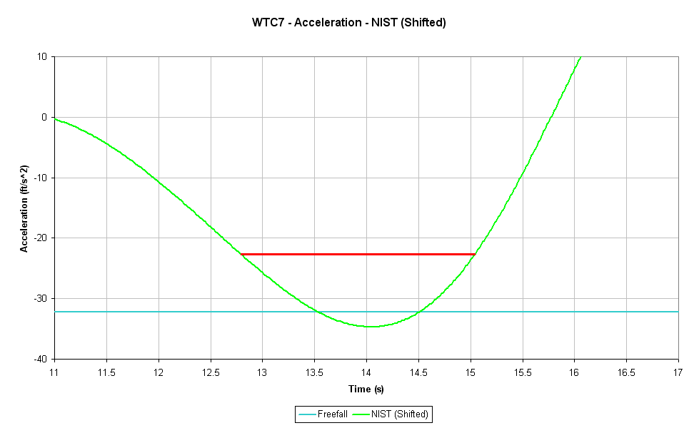
  • The reasoning behind my choice of T0 (11.71s) should be pretty obvious.
  • The curve implied by the NIST formula will clearly never correlate well with any of my curves over the full duration, no matter where you shift it to on the time axis.
  • The steep increase in acceleration shown by all of my graphs (and tfk's) shows what happened.
  • My graphs are not T0 dependant (as I have told you a few times).
Repeatedly suggesting ALL of my curves (and tfk's) are inaccurate between 11 and 13 seconds is based upon your particular method of determining accuracy, and must be where you are going wrong.

If your particular method (and procedure) spits out a number saying that the green curve is a better fit to the underlying data, then, sorry, but the method is flawed. That the green curve can be made to match for a short period is irrelevant to validating the NIST formula for the purpose of determining acceleration profile. (Or more likely, the numbers it spits out are meaningless in practice with noisy data)

Seriously: It's okay to disagree with NIST's choice of t=0. If you choose to regard a different moment as the beginning of the collapse, however, then you will have to adjust NIST's time-scaling parameter λ accordingly (and you will probably have to make slight adjustments to the other two parameters, A and k). In short, you will have to perform the same kind of least-squares minimization that NIST and I did.
See above. It does not matter where you shift the implied NIST acceleration curve. It will never be an even reasonable match to the truer acceleration profile (which emerges the same regardless of the many methods myself and tfk have used). You included a graph earlier with paramaters tuned to my data, and it would still never match to the actual trend.

One factor we must not forget...my data relates to the NW corner, NISTs to, well, somewhere else (see list of other NIST trace data issues).

Cavalier time-shifting of NIST's model without recalculating its parameters would be dishonest.
Do you mean like this...
the choice of 10.9 seconds as a reasonable offset between your time axis and NIST's
...and...
I came up with the 10.9 second offset by eyeball.

I have also chosen a T0 (11.71s) based upon the last point of inflexion of the S-B derived acceleration profile.

It is not a cavalier choice, but driven by observation of the data.

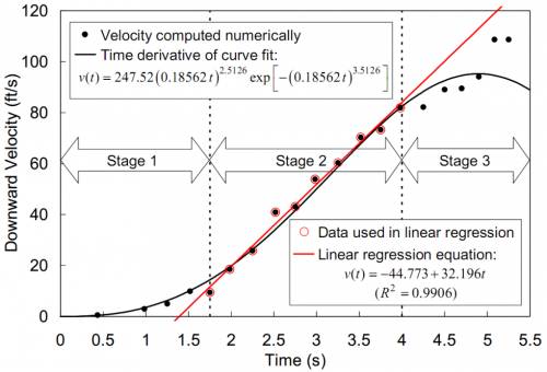
As you can see, that choice also fits consistently with the velocity and displacement data...
703997721.gif


Obviously it is necessary to place the NIST curve somewhere, though I do not see my own selection as being in the slightest bit cavalier. I could tend to think that of your own though.

Regardless, irrespective of where the implied NIST acceleration function curve is placed it will never be a good match, and your repeated assertions that it is more accurate during certain periods of time are simply a subjective and meaningless sum, which if you use a little cavalier eye-balling of the graphs, you can see for yourself.
 
Last edited by a moderator:
femr2 said:
irrespective of where the implied NIST acceleration function curve is placed it will never be a good match
In order to accomodate W.D.Clinger's viewpoint on alternate placement of the NIST function curves, here is the result of shifting them 60 frames (~1s) earlier (a 1s shift in T0)...

272520399.png

485183061.png

819970289.png


391373100.gif


As is expected both the displacement and velocity curves are a closer match, but, as I suggested above, the acceleration profile is still significantly different.

I have suggested on many occasions that I think NIST placed their T0 value about a second too early. I hope there is no longer much doubt about that relative to the NW corner.

I have highlighted that the *kink* does not form in the vertical direction and, as NIST defined their T0 relative to motion during the formation of the *kink*, I hope it is now clear why I make the assertion that NIST used an early T0.

I hope it is also now clear why erronious T0 definition has a large effect upon resultant calculated acceleration information.

A couple of questions to ask yourself:

  • Now that you have seen the implied NIST acceleration function, and its behaviour around g, would you suggest gravitational acceleration for 2.25s ?
  • Why did NIST not highlight that their function of motion exceeded g for ~1s ?
  • Why did NIST perform a linear regression to state acceleration (at 32.196ft/s^2 of all values) rather than use their model ?

I'd suggest NIST was fully aware that their derived acceleration curve was a poor fit.

I suggest they also wished to retain the "40% longer than freefall* metric.

A 1s change in T0 changes this metric to... 17% longer than *freefall*.

(If you agree with none of the above, then I suggest they simply didn't realise the mistake they'd made)
 
Last edited:
W.D.Clinger said:
The red line is NIST's linear approximation to part of NIST's nonlinear approximation.
...
You were telling us that your [acceleration] polynomials must be better than NIST's [acceleration] approximations because (you thought) NIST's [acceleration] approximations were linear.
...
you didn't realize that NIST's [acceleration] approximations were nonlinear
...
NIST's model of the acceleration is not a straight line.
...
NIST's models of displacement, velocity, and acceleration are all nonlinear.
...
NIST's velocity and acceleration models are immediate consequences (via freshman calculus) of that nonlinear model.
...
etc
Parentheses added by me for clarity of context.

A slight reminder on this point...

NIST only derived their displacement formula to velocity.

The only acceleration model used is the linear regression, and it is from that linear regression that their stated metrics are generated...

659040095.jpg


NIST used the datapoints circled in red (which were themselves determined by central difference approximation from the underlying displacement data) to calculate their stated linear regression (the red line)...

v(t) = -44.773 + 32.196t


It is this linear regression which is used to specify the rough 2.25s *freefall* period.

That fact is made even clearer if we actually look at the implied NIST acceleration function (which they did not use) and check the period of time which it can reasonably be said to approximate gravitational acceleration...
238197312.png


I have taken the liberty of marking a 2.25s duration in red and gravitational acceleration in cyan.
 
Last edited:
T-zero

W.D.Clinger said:
I came up with the 10.9 second offset by eyeball...If I am wrong, then fixing it would improve the accuracy of NIST's model without improving the accuracy of yours
...
it doesn't have anything at all to do with T0 or with the translation between NIST's time scale and yours, because the fact I stated is a fact about your Poly(10) approximation
...
I have not made any "personal choice of T0"...the choice of 10.9 seconds as a reasonable offset between your time axis and NIST's
...
My choice of 10.9 seconds cannot affect the computed accuracy of your model. A better choice for that offset can only improve the computed accuracy of NIST's model.
...
You are talking nonsense. Calculating the residual sum of squares for your models does not involve any notion of a T0.
...
P(t) will be a poor approximation to the time series at times t that are just outside the interval...I suspect that's why femr2's Poly(10) model is so inaccurate between 11 and 13 seconds
...
I trust that you now understand how the definition of T0 is highly relevant, not only with regards to your statements above, but to this discussion in general.

t=0 is by definition the T0 for the NIST formulas (naturally).

T0 for my data is a choice, but an informed choice places it at ~11.71s.

Therefore discussion in this context is about where the NIST curve is placed upon the time axis of my data.

Moving the NIST implied acceleration curve along the time axis of my acceleration graph has the direct implication of change in T0 for my data, which is why I have repeatedly highlighted that T0 cannot be ignored (an implication which you've called nonsense).

Given that change in T0 on my graph determines where the start of my curve is for the purposes of determining acceleration, it also has the effect of defining the portion of the Poly fits which extend above the zero line. (T0 for the NIST formula should really always be aligned with T0 on my data. That is why I have ensured that the graphs with a fudged NIST T0 are marked Shifted)

Given that your residual calculation included a significant period of time before my more correct T0, I hope you now understand why you were getting non-sensible accuracy results, and I hope you now understand why (given I have stated and justified T0 for my data) I disagree with you even at the level of residual calc in terms of accuracy. (You can of course test that if you like, by changing your 10.9s parameter to 11.71s and re-running your residual calcs)

Your choice of 10.9s defines the relative T0 for my data.

Do you still hold to your statements above ?
 
The NIST data suffers from the following (non-exhaustive) series of technical issues, each of which reduce the quality, validity and relevance of the data in various measures...

  • NIST did not deinterlace their source video. This has two main detrimental effects: 1) Each image they look at is actually a composite of two separate points in time, and 2) Instant halving of the number of frames available...half the available video data information. Tracing features using interlaced video is *not a good idea*. I have gone into detail on issues related to tracing of features using interlaced video data previously.
  • NIST did not sample every frame, reducing the sampling rate considerably and reducing available data redundancy for the purposes of noise reduction and derivation of velocity and acceleration profile data.
  • NIST used an inconsistent inter-sample time-step, skipping roughly every 56 out of 60 available frames. They ignored over 90% of the available frame data.
  • NIST likely used a manual (by hand-eye) tracking process using a single pixel column, rather than a tried and tested feature tracking method such as those provided in systems such as SynthEyes. Manual tracking introduces a raft of accuracy issues. Feature tracking systems such as SynthEyes employ an automated region-based system which entails upscaling of the target region, application of LancZos3 filtering and pattern matching (with FOM) to provide a sub-pixel accurate relative location of initial feature pattern in subsequent frames in video.
  • NIST tracked the *roofline* using a single pixel column, rather than an actual feature of the building. This means that the trace is not actually of a point of the building, as the building does not descend completely vertically. This means the tracked pixel column is actually a rather meaningless point on the roofline which wanders left and right as the building moves East and West.
  • NIST used the Cam#3 viewpoint which includes significant perspective effects (such as early motion being north-south rather than up-down and yet appearing to be vertical motion).
  • NIST did not perform perspective correction upon the resultant trace data.
  • NIST did not appear to recognise that the initial movement at their chosen pixel column was north-south movement resulting from twisting of the building before the release point of the north facade.
  • NIST did not perform static point extraction(H, V). Even when the camera appears static, there is still (at least) fine movement. Subtraction of static point movement from trace data significantly reduces camera shake noise, and so reduces track data noise.
  • NIST did not choose a track point which could actually be identified from the beginning to the end of the trace, and so they needed to splice together information from separate points. Without perspective correction the scaling metrics for these two points resulted in data skewing, especially of the early motion.

Having performed a fair bit of video feature tracking myself, most of the issues highlighted really should have been dealt with.

Needless to say I hope it is becoming clear why I do not hold the NIST motion data in high regard.

Most of these issues are unaffected by recent discussion.

If you disagree with any of these issues, by all means make it known, though I suggest discussing one issue at a time and making your objection clear and detailed.

Probably prudent to add to the list...

 
Last edited:
You've made some kind of mistake. If you compare the black curve in that graph with the red curve in the graph below, you'll see that they're offset by about a quarter of a second. Both of those graphs claim to be displaying your Poly(50) approximation. At least one of them must be wrong.
Damn. Yes, a trivial shift in time axis origin of 10 samples.

All of the recent graphs are shifted 10 samples (0.1668s) early. (add 0.1668s to each *vs* graph origin to realign it with raw data)

Trivial to sort in my local data, pain in the posterior to regenerate graphs. Hmm. If I get the time. I'd rather not have two copies. I can replace the existing images, but it will throw out T0 definitions within the thread :(
 
Last edited:
Errata

Okay, I've updated the *vs* images to correct the time axis shift slip-up.

Recent *vs* graph T0 references earlier in the thread should be: 11.88s (not 11.71s)
 
interval of time | NIST original | NIST tuned | Poly(10)
11 to 17 s | 14861 | 2879 | 4628
11 to 13 s | 962 | 428 | 4234
15 to 17 s | 12964 | 1751 | 296

...

The following graph displays the instantaneous velocity computed by central differencing, as described in NIST section 12.5.3, with absolutely no smoothing of position or velocity. (I didn't want to run the risk that my choice of smoothing algorithm might favor one of the models being compared.) Once again, you can see that most of the error in the NIST-style models comes after 16 seconds.

danV.png

A couple of questions I hinted at earlier, but then forgot to actually ask...

  1. What derivative do your SSerr values relate to: velocity or acceleration ?
  2. If acceleration, did you simply apply another central difference approximation to the derived velocity data ?
  3. Did you use adjacent samples in my data when performing central difference approximation, or a wider band equivalent to the NIST ~0.25s sample interval ?
 
Femr, is this a place to discuss the interpretation of the drop and acceleration data?

The meaning of the "greater than g" hump in the data?
 

Back
Top Bottom